Example 8: Particle motion in two dimensions

In this example we will calculate the motion of a particle in two dimensions. First we will calculate the motion of a smooth ball with drag coefficient given by the previously defined function cd_sphere() (see Example 2: Sphere in free fall), and then of a golf ball with drag and lift.

The problem is illustrated in the following figure:

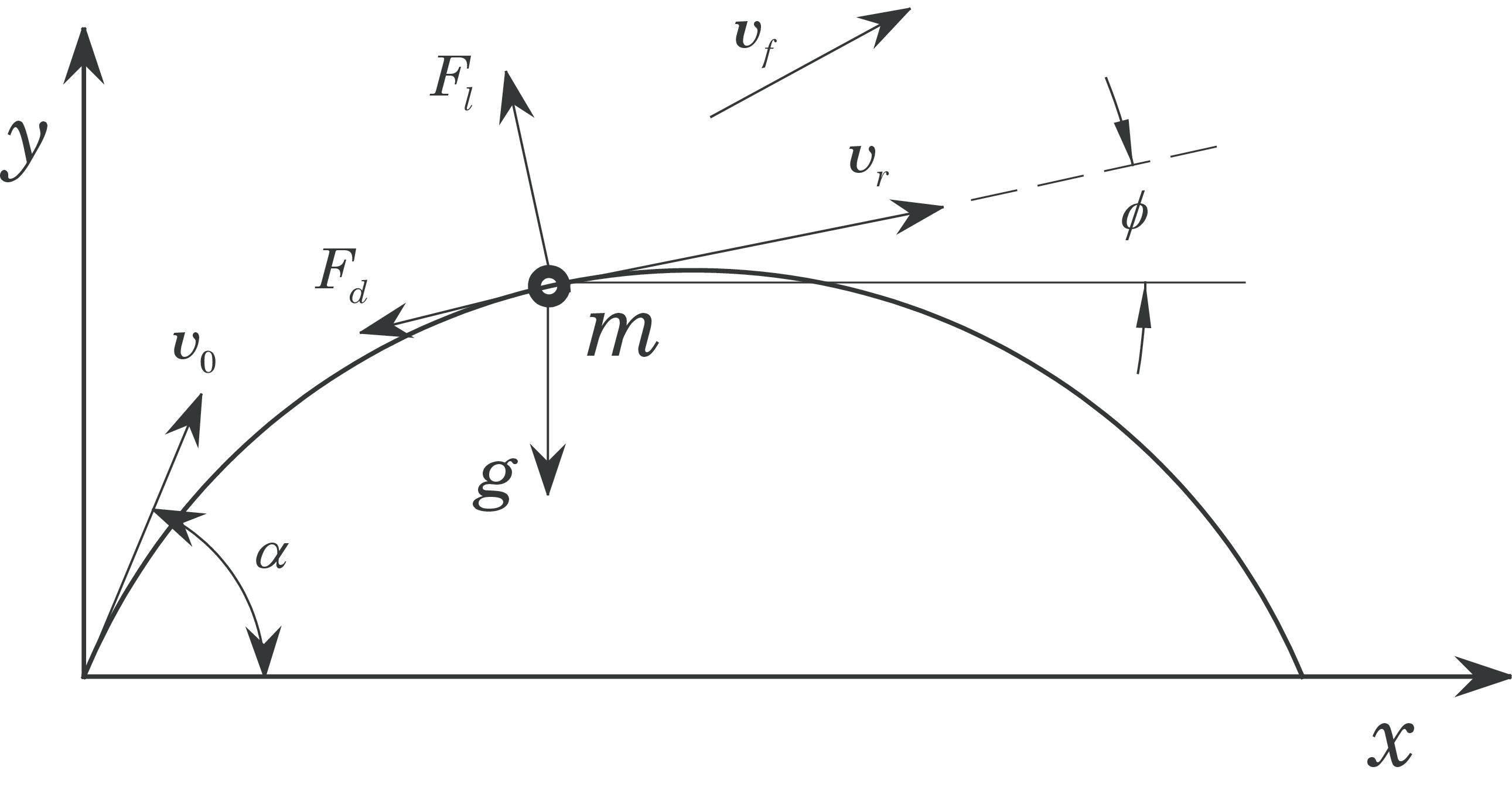
where \( v \) is the absolute velocity, \( v_f= \) is the velocity of the fluid, \( v_r=v-v_f \) is the relative velocity between the fluid and the ball, \( \alpha \) is the elevation angle, \( v_0 \) is the initial velocity and \( \phi \) is the angle between the \( x \)-axis and \( v_r \).

\( \mathbf{F}_l \) is the lift force stemming from the rotation of the ball (the Magnus-effect) and is normal to \( v_r \). With the given direction the ball rotates counter-clockwise (backspin). \( \mathbf{F}_d \) is the fluids resistance against the motion and is parallel to \( v_r \). These forces are given by $$ \begin{align} \mathbf{F}_d=\frac{1}{2}\rho _f AC_Dv_r^2 \tag{64}\\ \mathbf{F}_l=\frac{1}{2}\rho _f AC_Lv_r^2 \tag{65} \end{align} $$

\( C_D \) is the drag coefficient, \( C_L \) is the lift coefficient, \( A \) is the area projected in the velocity direction and \( \rho_F \) is the density of the fluid.

Newton's law in \( x \)- and \( y \)-directions gives $$ \begin{align} \tag{66} \frac{dv_x}{dt}&= -\rho _f\frac{A}{2m}v_r^2(C_D\cdot \cos(\phi)+C_L\sin(\phi)) \\ \frac{dv_y}{dt}&=\rho _f\frac{A}{2m}v_r^2(C_L\cdot \cos(\phi)-C_D\sin(\phi))-g \tag{67} \end{align} $$

From the figure we have $$ \begin{align*} \cos (\phi)&=\frac{v_{rx}}{v_r} \\ \sin(\phi)&=\frac{v_{ry}}{v_r} \end{align*} $$

We assume that the particle is a sphere, such that \( C=\rho _f\frac{A}{2m}=\frac{3\rho_f}{4\rho_kd} \) as in (Example 2: Sphere in free fall). Here \( d \) is the diameter of the sphere and \( \rho_k \) the density of the sphere.

Now (66) and (67) become $$ \begin{align} \tag{68} \frac{dv_x}{dt} &= -C\cdot v_r(C_D\cdot v_{rx}+C_L\cdot v_{ry})\\ \frac{dv_y}{dt} &= C\cdot v_r(C_L\cdot v_{rx}-C_D\cdot v_{ry})- \tag{69}g \end{align} $$

With \( \frac{dx}{dt}=v_x \) and \( \frac{dy}{dt}=v_y \) we get a system of 1st order equations as follows, $$ \begin{align} &\frac{dx}{dt}=v_x \nonumber \\ & \frac{dy}{dt}=v_y \nonumber\\ & \frac{dv_x}{dt} = -C\cdot v_r(C_D\cdot v_{rx}+C_L\cdot v_{ry}) \tag{70}\\ &\frac{dv_y}{dt} = C\cdot v_r(C_L\cdot v_{rx}-C_D\cdot v_{ry})-g \nonumber \end{align} $$

Introducing the notation \( x=y_1 \), \( y=y_2 \), \( v_x=y_3 \), \( v_y=y_4 \), we get $$ \begin{align} &\frac{dy_1}{dt}=y_3\nonumber\\ & \frac{dy_2}{dt}=y_4\nonumber\\ & \frac{dy_3}{dt} = -C\cdot v_r(C_D\cdot v_{rx}+C_L\cdot v_{ry}) \tag{71}\\ &\frac{dy_4}{dt} = C\cdot v_r(C_L\cdot v_{rx}-C_D\cdot v_{ry})-g\nonumber \end{align} $$

Here we have \( v_{rx}=v_x-v_{fx}=y_3-v_{fx},\ v_{ry}=v_y-v_{fy}=y_4-v_{fy},\\ v_r=\sqrt{v_{rx}^2+v_{ry}^2} \)

Initial conditions for \( t=0 \) are $$ \begin{align*} y_1&=y_2=0 \\ y_3&=v_0\cos(\alpha)\\ y_4&=v_0\sin(\alpha) \end{align*} $$

Let's first look at the case of a smooth ball. We use the following data (which are the data for a golf ball): $$ \begin{equation*} \tag{72} \text{Diameter } d = 41 \text{mm},\text{ mass } m = 46\text{g which gives } \rho_k=\frac{6m}{\pi d^3} = 1275 \text{kg/m}^3 \end{equation*} $$ We use the initial velocity \( v_0=50 \) m/s and solve (71) using the Runge-Kutta 4 scheme. In this example we have used the Python package Odespy (ODE Software in Python), which offers a large collection of functions for solving ODE's. The RK4 scheme available in Odespy is used herein.

The right hand side in (71) is implemented as the following function:

def f(z, t):
    """4x4 system for smooth sphere with drag in two directions."""
    zout = np.zeros_like(z)
    C = 3.0*rho_f/(4.0*rho_s*d)
    vrx = z[2] - vfx
    vry = z[3] - vfy
    vr = np.sqrt(vrx**2 + vry**2)
    Re = vr*d/nu
    CD = cd_sphere(Re) # using the already defined function
    zout[:] = [z[2], z[3], -C*vr*(CD*vrx), C*vr*(-CD*vry) - g]

Note that we have used the function cd_sphere() defined in (Example 2: Sphere in free fall) to calculate the drag coefficient of the smooth sphere.

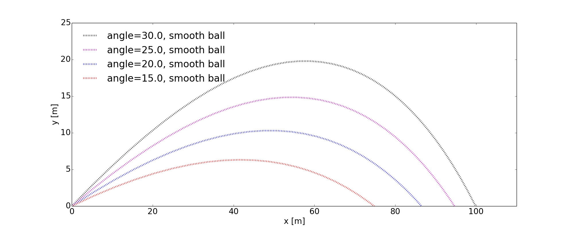
The results are shown for some initial angles in Figure 11.

Now let's look at the same case for a golf ball. The dimension and weight are the same as for the sphere. Now we need to account for the lift force from the spin of the ball. In addition, the drag data for a golf ball are completely different from the smooth sphere. We use the data from Bearman and Harvey [6] who measured the drag and lift of a golf ball for different spin velocities in a vindtunnel. We choose as an example 3500 rpm, and an initial velocity of \( v_0=50 \) m/s.

The right hand side in (71) is now implemented as the following function:

def f3(z, t):
    """4x4 system for golf ball with drag and lift in two directions."""
    zout = np.zeros_like(z)
    C = 3.0*rho_f/(4.0*rho_s*d)
    vrx = z[2] - vfx
    vry = z[3] - vfy
    vr = np.sqrt(vrx**2 + vry**2)
    Re = vr*d/nu
    CD, CL = cdcl(vr, nrpm)
    zout[:] = [z[2], z[3], -C*vr*(CD*vrx + CL*vry), C*vr*(CL*vrx - CD*vry) - g]

The function cdcl() (may be downloaded here) gives the drag and lift data for a given velocity and spin.

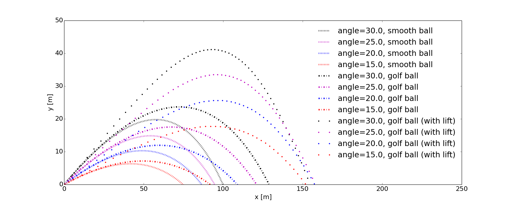
The results are shown in Figure 12. The motion of a golf ball with drag but without lift is also included. We see that the golf ball goes much farther than the smooth sphere, due to less drag and the lift.

The complete program ParticleMotion2D.py is listed below.

# chapter1/programs_and_modules/ParticleMotion2D.py;DragCoefficientGeneric.py @ git@lrhgit/tkt4140/allfiles/digital_compendium/chapter1/programs_and_modules/DragCoefficientGeneric.py;cdclgolfball.py @ git@lrhgit/tkt4140/allfiles/digital_compendium/chapter1/programs_and_modules/cdclgolfball.py;

from DragCoefficientGeneric import cd_sphere
from cdclgolfball import cdcl  
from matplotlib.pyplot import *
import numpy as np
import odespy

g = 9.81      # Gravity [m/s^2]
nu = 1.5e-5   # Kinematical viscosity [m^2/s]
rho_f = 1.20  # Density of fluid [kg/m^3]
rho_s = 1275  # Density of sphere [kg/m^3]
d = 41.0e-3   # Diameter of the sphere [m]
v0 = 50.0     # Initial velocity [m/s]
vfx = 0.0     # x-component of fluid's velocity
vfy = 0.0     # y-component of fluid's velocity

nrpm = 3500   # no of rpm of golf ball

# smooth ball
def f(z, t):
    """4x4 system for smooth sphere with drag in two directions."""
    zout = np.zeros_like(z)
    C = 3.0*rho_f/(4.0*rho_s*d)
    vrx = z[2] - vfx
    vry = z[3] - vfy
    vr = np.sqrt(vrx**2 + vry**2)
    Re = vr*d/nu
    CD = cd_sphere(Re) # using the already defined function
    zout[:] = [z[2], z[3], -C*vr*(CD*vrx), C*vr*(-CD*vry) - g]
    return zout 

# golf ball without lift
def f2(z, t):
    """4x4 system for golf ball with drag in two directions."""
    zout = np.zeros_like(z)
    C = 3.0*rho_f/(4.0*rho_s*d)
    vrx = z[2] - vfx
    vry = z[3] - vfy
    vr = np.sqrt(vrx**2 + vry**2)
    Re = vr*d/nu
    CD, CL = cdcl(vr, nrpm)
    zout[:] = [z[2], z[3], -C*vr*(CD*vrx), C*vr*(-CD*vry) - g]
    return zout 

# golf ball with lift
def f3(z, t):
    """4x4 system for golf ball with drag and lift in two directions."""
    zout = np.zeros_like(z)
    C = 3.0*rho_f/(4.0*rho_s*d)
    vrx = z[2] - vfx
    vry = z[3] - vfy
    vr = np.sqrt(vrx**2 + vry**2)
    Re = vr*d/nu
    CD, CL = cdcl(vr, nrpm)
    zout[:] = [z[2], z[3], -C*vr*(CD*vrx + CL*vry), C*vr*(CL*vrx - CD*vry) - g]
    return zout 


# main program starts here

T = 7   # end of simulation
N = 60  # no of time steps
time = np.linspace(0, T, N+1)

N2 = 4
alfa = np.linspace(30, 15, N2)   # Angle of elevation [degrees]
angle = alfa*np.pi/180.0 # convert to radians

legends=[]
line_color=['k','m','b','r']
figure(figsize=(20, 8))
hold('on')
LNWDT=4; FNT=18
rcParams['lines.linewidth'] = LNWDT; rcParams['font.size'] = FNT

# computing and plotting

# smooth ball with drag
for i in range(0,N2):
    z0 = np.zeros(4)
    z0[2] = v0*np.cos(angle[i])
    z0[3] = v0*np.sin(angle[i])
    solver = odespy.RK4(f)
    solver.set_initial_condition(z0)
    z, t = solver.solve(time)
    plot(z[:,0], z[:,1], ':', color=line_color[i])
    legends.append('angle='+str(alfa[i])+', smooth ball')
    
# golf ball with drag
for i in range(0,N2):
    z0 = np.zeros(4)
    z0[2] = v0*np.cos(angle[i])
    z0[3] = v0*np.sin(angle[i])
    solver = odespy.RK4(f2)
    solver.set_initial_condition(z0)
    z, t = solver.solve(time)
    plot(z[:,0], z[:,1], '-.', color=line_color[i])
    legends.append('angle='+str(alfa[i])+', golf ball')
     
# golf ball with drag and lift
for i in range(0,N2):
    z0 = np.zeros(4)
    z0[2] = v0*np.cos(angle[i])
    z0[3] = v0*np.sin(angle[i])
    solver = odespy.RK4(f3)
    solver.set_initial_condition(z0)
    z, t = solver.solve(time)
    plot(z[:,0], z[:,1], '.', color=line_color[i])
    legends.append('angle='+str(alfa[i])+', golf ball (with lift)')
 
legend(legends, loc='best', frameon=False)
xlabel('x [m]')
ylabel('y [m]')
axis([0, 250, 0, 50])
savefig('example_particle_motion_2d_2.png', transparent=True)
show()