Numerical Methods for Engineers

Example 4: Numerical error as a function of $ \Delta t $

In this example we will assess how the error of our implementation of the Euler method depends on the time step $ \Delta t $ in a systematic manner. We will solve a problem with an analytical solution in a loop, and for each new solution we do the following:

Divide the time step by two (or double the number of time steps)
Compute the error
Plot the error

Euler's method is a first order method and we expect the error to be $ O(h)=O(\Delta t) $. Consequently if the timestep is divided by two, the error should also be divided by two. As errors normally are small values and are expected to be smaller and smaller for decreasing time steps, we normally do not plot the error itself, but rather the logarithm of the absolute value of the error. The latter we do due to the fact that we are only interested in the order of magnitude of the error, whereas errors may be both positive and negative. As the initial value is always correct we discard the first error at time zero to avoid problems with the logarithm of zero in log_error = np.log10(abs_error[1:]).

# chapter1/programs_and_modules/Euler_timestep_ctrl.py;DragCoefficientGeneric.py @ git@lrhgit/tkt4140/allfiles/digital_compendium/chapter1/programs_and_modules/DragCoefficientGeneric.py;
from DragCoefficientGeneric import cd_sphere    
from matplotlib.pyplot import *
import numpy as np

# change some default values to make plots more readable 
LNWDT=5; FNT=11
rcParams['lines.linewidth'] = LNWDT; rcParams['font.size'] = FNT
font = {'size' : 16}; rc('font', **font)



g = 9.81      # Gravity m/s^2
d = 41.0e-3   # Diameter of the sphere
rho_f = 1.22  # Density of fluid [kg/m^3]
rho_s = 1275  # Density of sphere [kg/m^3]
nu = 1.5e-5   # Kinematical viscosity [m^2/s]
CD = 0.4      # Constant drag coefficient

def f(z, t):
    """2x2 system for sphere with constant drag."""
    zout = np.zeros_like(z)
    alpha = 3.0*rho_f/(4.0*rho_s*d)*CD
    zout[:] = [z[1], g - alpha*z[1]**2]
    return zout 

# define euler scheme
def euler(func,z0, time):
    """The Euler scheme for solution of systems of ODEs. 
    z0 is a vector for the initial conditions, 
    the right hand side of the system is represented by func which returns 
    a vector with the same size as z0 ."""
    
    z = np.zeros((np.size(time),np.size(z0)))
    z[0,:] = z0

    for i in range(len(time)-1):
        dt = time[i+1]-time[i]
        z[i+1,:]=z[i,:] + np.asarray(func(z[i,:],time[i]))*dt
    return z

def v_taylor(t):
#    z = np.zeros_like(t)
    v = np.zeros_like(t)
    alpha = 3.0*rho_f/(4.0*rho_s*d)*CD
    v=g*t*(1-alpha*g*t**2)
    return v
     
# main program starts here

T = 10  # end of simulation
N = 10  # no of time steps


z0=np.zeros(2)
z0[0] = 2.0

# Prms for the analytical solution 
k1 = np.sqrt(g*4*rho_s*d/(3*rho_f*CD))
k2 = np.sqrt(3*rho_f*g*CD/(4*rho_s*d))

Ndts = 4  # Number of times to divide the dt by 2 
legends=[]
error_diff = []

for i in range(Ndts+1):
    time = np.linspace(0, T, N+1)
    ze = euler(f, z0, time)     # compute response with constant CD using Euler's method
    v_a = k1*np.tanh(k2*time)   # compute response with constant CD using analytical solution
    abs_error=np.abs(ze[:,1] - v_a)
    log_error = np.log10(abs_error[1:])
    max_log_error = np.max(log_error)
    #plot(time, ze[:,1])
    plot(time[1:], log_error)
    legends.append('Euler scheme: N ' + str(N) + ' timesteps' )
    N*=2
    if i > 0:
        error_diff.append(previous_max_log_err-max_log_error)

    previous_max_log_err = max_log_error
    
print 10**(np.mean(error_diff)), np.mean(error_diff)


# plot analytical solution
# plot(time,v_a)
# legends.append('analytical')

# fix plot 
legend(legends, loc='best', frameon=False)
xlabel('Time [s]')
#ylabel('Velocity [m/s]')
ylabel('log10-error')
savefig('example_euler_timestep_study.png', transparent=True)
show()

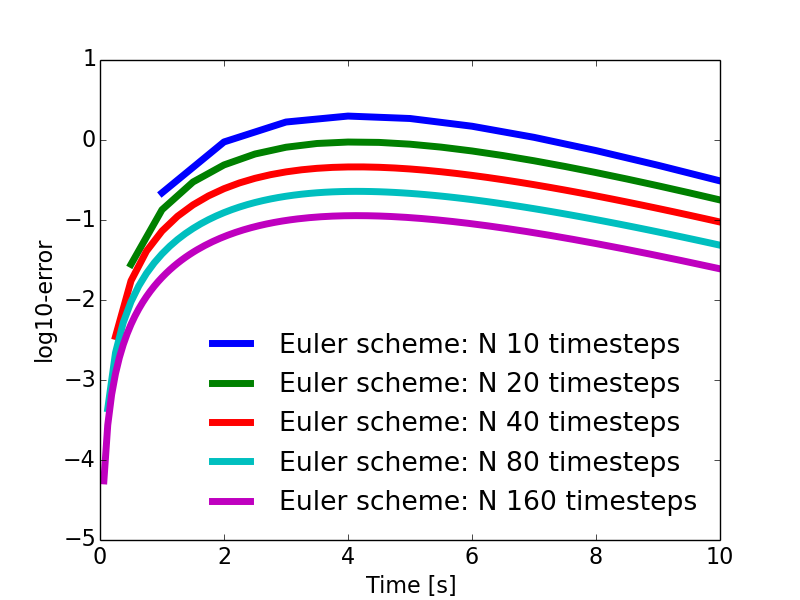
The plot resulting from the code above is shown in Figure (5). The difference or distance between the curves seems to be rather constant after an initial transient. As we have plotted the logarithm of the absolute value of the error $ \epsilon_i $, the difference $ d_{i+1} $ between two curves is $ d_{i+1}= \log10 \epsilon_{i}-\log10 \epsilon_{i+1} = \displaystyle \log10 \frac{\epsilon_{i}}{\epsilon_{i+1}} $. A rough visual inspection of Figure (5) yields $ d_{i+1} \approx 0.3 $, from which we may deduce: $$ \begin{equation} \log10 \frac{\epsilon_{i}}{\epsilon_{i+1}} \approx 0.3 \Rightarrow \epsilon_{i+1} \approx 10^{-0.3}\, \epsilon_{i} \approx 0.501\, \epsilon_{i} \tag{47} \end{equation} $$

The print statement print 10**(np.mean(error_diff)), np.mean(error_diff) returns 2.04715154702 0.311149993907, thus we see that the error is reduced even slightly more than the theoretically expected value for a first order scheme, i.e. $ \Delta t_{i+1} = \Delta t_{i}/2 $ yields $ \epsilon_{i+1} \approx\epsilon_{i}/2 $.

Figure 5: Plots for the logarithmic errors for a falling sphere with constant drag. The timestep $ \Delta t $ is reduced by a factor two from one curve to the one immediately below.

Example 4: Numerical error as a function of \( \Delta t \)