Example 6: Falling sphere with Heun's method
Let's go back to (Example 3: Falling sphere with constant and varying drag), and implement a new function heun() in the program FallingSphereEuler.py.
We recall the system of equations as $$ \begin{align*} &\frac{dz}{dt}=v\\ &\frac{dv}{dt}=g-\alpha v^2 \end{align*} $$ which by use of Heun's method in (58) and (59) becomes
Predictor: $$ \begin{align} z^p_{n+1}&=z_n+\Delta t v_n \\ v^p_{n+1}&= v_n +\Delta t \cdot (g-\alpha v^2_n) \nonumber \end{align} $$ Corrector: $$ \begin{align} z_{n+1}&=z_n+0.5\Delta t \cdot (v_n+v^p_{n+1}) \\ v_{n+1}&=v_n+0.5\Delta t \cdot \left[2g-\alpha[v^2_n+(v^p_{n+1})^2\right] \nonumber \end{align} $$ with initial values \( z_0=z(0)=0,\ v_0=v(0)=0 \). Note that we don't use the predictor \( z^p_{n+1} \) since it doesn't appear on the right hand side of the equation system.
One possible way of implementing this scheme is given in the following function named heun(), in the program ODEschemes.py:
def heun(func, z0, time):
    """The Heun scheme for solution of systems of ODEs.
    z0 is a vector for the initial conditions,
    the right hand side of the system is represented by func which returns
    a vector with the same size as z0 ."""

    def f_np(z,t):
        """A local function to ensure that the return of func is an np array
        and to avoid lengthy code for implementation of the Heun algorithm"""
        return np.asarray(func(z,t))

    z = np.zeros((np.size(time), np.size(z0)))
    z[0,:] = z0
    zp = np.zeros_like(z0)

    for i, t in enumerate(time[0:-1]):
        dt = time[i+1] - time[i]
        zp = z[i,:] + f_np(z[i,:],t)*dt   # Predictor step
        z[i+1,:] = z[i,:] + (f_np(z[i,:],t) + f_np(zp,t+dt))*dt/2.0 # Corrector step
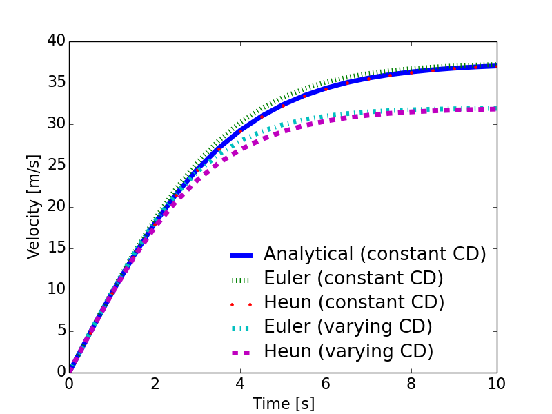
Using the same time steps as in (Example 3: Falling sphere with constant and varying drag), we get the response plotted in Figure 8.
Figure 8: Velocity of falling sphere using Euler's and Heun's methods.
The complete program FallingSphereEulerHeun.py is listed below. Note that the solver functions euler and heun are imported from the script ODEschemes.py.
# chapter1/programs_and_modules/FallingSphereEulerHeun.py;ODEschemes.py @ git@lrhgit/tkt4140/allfiles/digital_compendium/chapter1/programs_and_modules/ODEschemes.py;
from DragCoefficientGeneric import cd_sphere
from ODEschemes import euler, heun
from matplotlib.pyplot import *
import numpy as np

# change some default values to make plots more readable
LNWDT=5; FNT=11
rcParams['lines.linewidth'] = LNWDT; rcParams['font.size'] = FNT

g = 9.81      # Gravity m/s^2
d = 41.0e-3   # Diameter of the sphere
rho_f = 1.22  # Density of fluid [kg/m^3]
rho_s = 1275  # Density of sphere [kg/m^3]
nu = 1.5e-5   # Kinematical viscosity [m^2/s]
CD = 0.4      # Constant drag coefficient

def f(z, t):
    """2x2 system for sphere with constant drag."""
    zout = np.zeros_like(z)
    alpha = 3.0*rho_f/(4.0*rho_s*d)*CD
    zout[:] = [z[1], g - alpha*z[1]**2]
    return zout

def f2(z, t):
    """2x2 system for sphere with Re-dependent drag."""
    zout = np.zeros_like(z)
    v = abs(z[1])
    Re = v*d/nu
    CD = cd_sphere(Re)
    alpha = 3.0*rho_f/(4.0*rho_s*d)*CD
    zout[:] = [z[1], g - alpha*z[1]**2]
    return zout

# main program starts here

T = 10  # end of simulation
N = 20  # no of time steps
time = np.linspace(0, T, N+1)

z0=np.zeros(2)
z0[0] = 2.0

ze = euler(f, z0, time)     # compute response with constant CD using Euler's method
ze2 = euler(f2, z0, time)   # compute response with varying CD using Euler's method

zh = heun(f, z0, time)     # compute response with constant CD using Heun's method
zh2 = heun(f2, z0, time)   # compute response with varying CD using Heun's method

k1 = np.sqrt(g*4*rho_s*d/(3*rho_f*CD))
k2 = np.sqrt(3*rho_f*g*CD/(4*rho_s*d))
v_a = k1*np.tanh(k2*time)   # compute response with constant CD using analytical solution

# plotting

legends=[]
line_type=['-',':','.','-.','--']

plot(time, v_a, line_type[0])
legends.append('Analytical (constant CD)')

plot(time, ze[:,1], line_type[1])
legends.append('Euler (constant CD)')

plot(time, zh[:,1], line_type[2])
legends.append('Heun (constant CD)')

plot(time, ze2[:,1], line_type[3])
legends.append('Euler (varying CD)')

plot(time, zh2[:,1], line_type[4])
legends.append('Heun (varying CD)')

legend(legends, loc='best', frameon=False)
font = {'size' : 16}
rc('font', **font)
xlabel('Time [s]')
ylabel('Velocity [m/s]')
savefig('example_sphere_falling_euler_heun.png', transparent=True)
show()