Heun's method
From (19) or (23) we have $$ \begin{equation} \tag{54} y''(x_n,y_n)=f'\left(x_n,y(x_n,y_n)\right)\approx \frac{f(x_n+h)-f(x_n)}{h} \end{equation} $$ The Taylor series expansion (17) gives $$ \begin{equation*} y(x_n+h)=y(x_n)+hy'[x_n,y(x_n)]+\frac{h^2}{2}y''[x_n,y(x_n)]+O(h^3) \end{equation*} $$ which, inserting (54), gives $$ \begin{equation} \tag{55} y_{n+1}=y_n+\frac{h}{2}\cdot [f(x_n,y_n)+f(x_{n+1},y(x_{n+1}))] \end{equation} $$
This formula is called the trapezoidal formula, since it reduces to computing an integral with the trapezoidal rule if \( f(x,y) \) is only a function of \( x \). Since \( y_{n+1} \) appears on both sides of the equation, this is an implicit formula which means that we need to solve a system of non-linear algebraic equations if the function \( f(x,y) \) is non-linear. One way of making the scheme explicit is to use the Euler scheme (41) to calculate \( y(x_{n+1}) \) on the right side of (55). The resulting scheme is often denoted Heun's method.
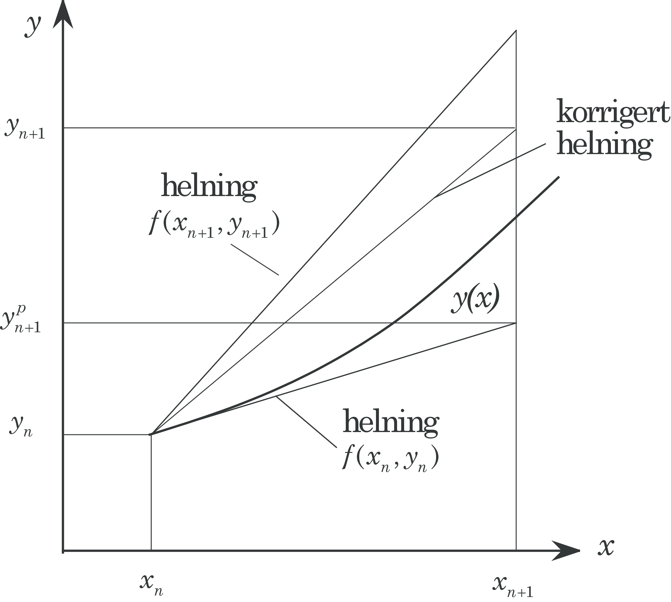
The scheme for Heun's method becomes $$ \begin{align} &y^p_{n+1}=y_n+h\cdot f(x_n,y_n) \tag{56} \\ &y_{n +1}=y_n+\frac{h}{2}\cdot[f(x_n,y_n)+f(x_{n+1},y^p_{n+1})] \tag{57} \end{align} $$ Index \( p \) stands for "predicted". (56) is then the predictor and (57) is the corrector. This is a second order method. For more details, see [5]. Figure 6 is a graphical illustration of the method.
Figure 6: Illustration of Heun's method.
In principle we could make an iteration procedure where we after using the corrector use the corrected values to correct the corrected values to make a new predictor and so on. This will likely lead to a more accurate solution of the difference scheme, but not necessarily of the differential equation. We are therefore satisfied by using the corrector once. For a system, we get $$ \begin{align} & \mathbf{y^p_{n+1}}=\mathbf{y_n}+h\cdot \mathbf{f}(x_n,\mathbf{y_n}) \tag{58}\\ & \mathbf{y_{n+1}}=\mathbf{y_n} +\frac{h}{2}\cdot [\mathbf{f}(x_n,\mathbf{y_n})+\mathbf{f}(x_{n+1},\mathbf{y^p_{n+1}})] \tag{59} \end{align} $$ Note that \( \mathbf{y}^p_{n+1} \) is a temporary variable that is not necessary to store.
If we use (58) and (59) on the example in (52) we get
Predictor: $$ \begin{align*} (y_1)^p_{n+1}&=(y_1)_n+h\cdot (y_2)_n&\\ (y_2)^p_{n+1}&=(y_2)_n+h\cdot (y_3)_n&\\ (y_3)^p_{n+1}&=(y_3)_n-h\cdot (y_1)_n\cdot (y_3)_n \end{align*} $$ Corrector: $$ \begin{align*} (y_1)_{n+1}&=(y_1)_n+0.5h\cdot [(y_2)_n+(y_2)^p_{n+1}]&\\ (y_2)_{n+1}&=(y_2)_n+0.5h\cdot [(y_3)_n+(y_3)^p_{n+1}]&\\ (y_3)_{n+1}&=(y_3)_n-0.5h\cdot [(y_1)_n\cdot (y_3)_n+(y_1)^p_{n+1}\cdot (y_3)^p_{n+1}] \end{align*} $$