Chapter 1: Initial value problems for Ordinary Differential Equations
Introduction
With an initial value problem for an ordinary differential equation (ODE) we mean a problem where all boundary conditions are given for one and the same value of the independent variable. For a first order ODE we get e.g. $$ \begin{align} \tag{1} y'(x)&=f(x,y) \\ y(x_0)&=a \nonumber \end{align} $$ while for a second order ODE we get $$ \begin{align} \tag{2} y''(x)&=f(x,y,y') \\ y(x_0)&=a,\ y'(x_0) = b \nonumber \end{align} $$ A first order ODE, as shown in Equation (1), will always be an initial value problem. For Equation (2), on the other hand, we can for instance specify the boundary conditions as follows, $$ \begin{align} y(x_0)=a,\ y(x_1) = b \nonumber \end{align} $$ With these boundary conditions Equation (2) presents a boundary value problem. In many applications boundary value problems are more common than initial value problems. But the solution technique for initial value problems may often be applied to solve boundary value problems.
Both from an analytical and numerical viewpoint initial value problems are easier to solve than boundary value problems, and methods for solution of initial value problems are more developed than for boundary value problems.
If we are to solve an initial value problem of the type in Equation (1), we must first be sure that it has a solution. In addition we will demand that this solution is unique, together the two criteria above lead to the following criteria:
A sufficient criteria for existence and uniqueness of a solution of the problem in Equation (1) is that both \( f(x,y) \) and \( \frac{\partial f}{\partial y} \) are continuous in and around \( x_0 \).
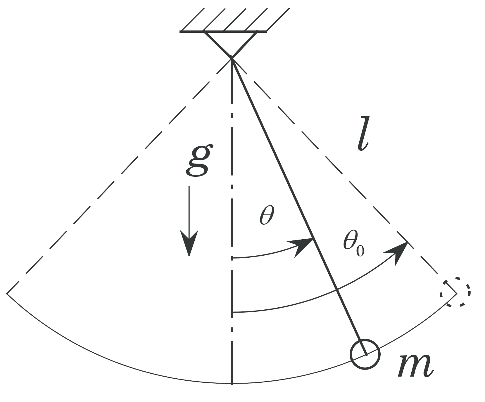
The figure shows a mathematical pendulum where the motion is described by the following equation: $$ \begin{align} \frac{\partial^2 \theta}{\partial \tau^2} + \frac{g}{l}\sin (\theta) = 0 \tag{3}\\ \theta (0) = \theta_0 ,\ \frac{d\theta}{d\tau}(0) = 0 \tag{4} \end{align} $$ We introduce a dimensionless time \( t \) given by \( t=\sqrt{\frac{g}{l}}\cdot\tau \) such that (3) and (4) may be written as $$ \begin{align} \tag{5} \ddot{\theta}(t) + \sin (\theta (t)) = 0 \\ \theta (0) = \theta_0 ,\ \dot\theta (0) = 0 \tag{6} \end{align} $$ The dot denotes derivation with respect to the dimensionless time \( t \). For small displacements we can set \( \sin (\theta) \approx \theta \), such that (5) and (6) becomes $$ \begin{align} \tag{7} \ddot\theta (t)& + \theta (t) = 0 \\ \theta (0)& = \theta_0 ,\ \dot\theta (0) = 0 \tag{8} \end{align} $$
The difference between (5) and (7) is that the latter is linear, while the first is non-linear. The analytical solution of Equations (5) and (6) is given in Appendix G.2. in the compendium. An \( n \)'th order linear ODE may be written on the form $$ \begin{equation} \tag{9} a_n(x)y^{(n)}(x)+a_{n-1}(x)y^{(n-1)}(x)+\cdots+a_1(x)y'(x)+a_0(x)y(x)=b(x) \end{equation} $$ where \( y^{(k)}, k=0,1,\dots n \) is referring to the \( k \)'th derivative and \( y^{(0)}(x)=y(x) \).
If one or more of the coefficients \( a_k \) also are functions of at least one \( y^{(k)},\ k = 0,1,\dots n \), the ODE is non-linear. From (9) it follows that (5) is non-linear and (7) is linear.
Analytical solutions of non-linear ODEs are rare, and except from some special types, there are no general ways of finding such solutions. Therefore non-linear equations must usually be solved numerically. In many cases this is also the case for linear equations. For instance it doesn't exist a method to solve the general second order linear ODE given by $$ \begin{equation} a_2(x)\cdot y''(x)+a_1(x)\cdot y'(x) +a_0(x)\cdot y(x) =b(x)\nonumber \end{equation} $$
From a numerical point of view the main difference between linear and non-linear equations is the multitude of solutions that may arise when solving non-linear equations. In a linear ODE it will be evident from the equation if there are special critical points where the solution change character, while this is often not the case for non-linear equations.
For instance the equation \( y'(x)=y^2(x),\ y(0)=1 \) has the solution \( y(x)=\frac{1}{1-x} \) such that \( y(x) \to \infty \) for \( x \to 1 \), which isn't evident from the equation itself.