Example 2: Sphere in free fall

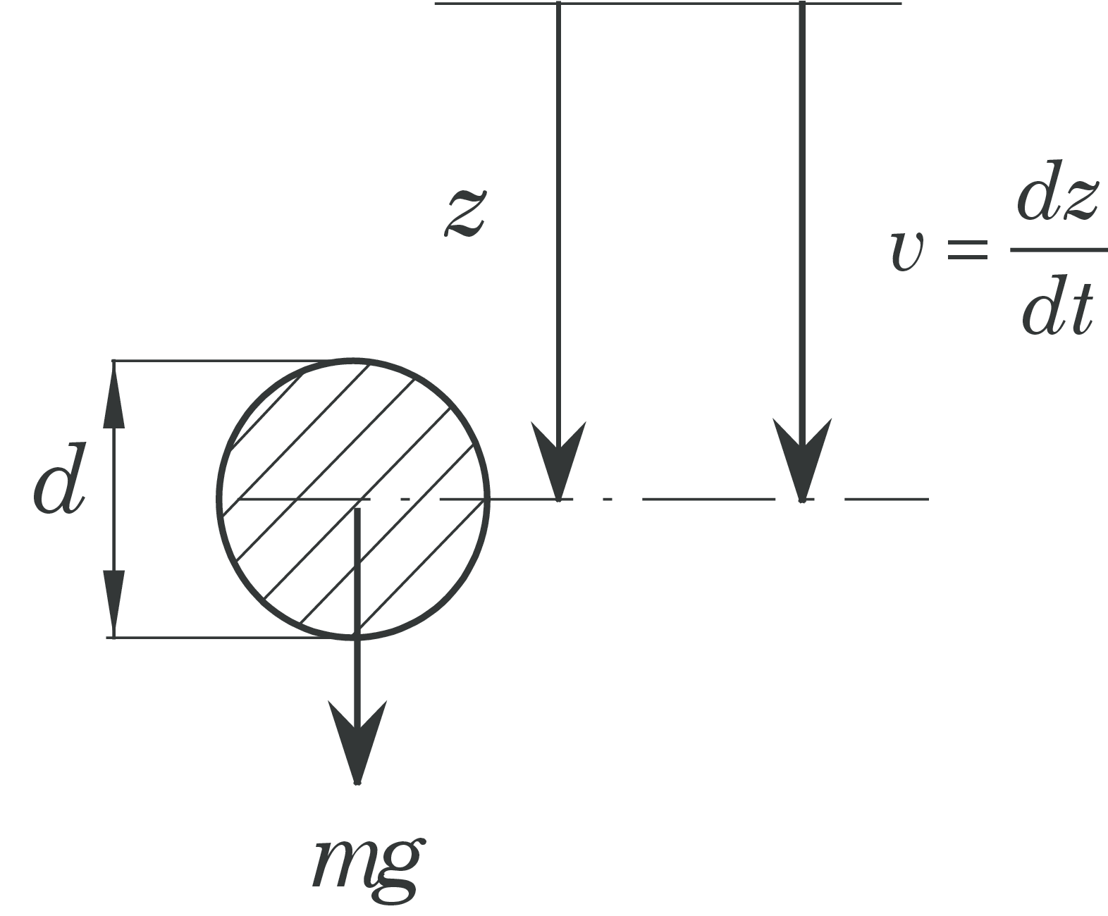
The figure shows a falling sphere with a diameter \( d \) and mass \( m \) that falls vertically in a fluid. Use of Newton's 2nd law in the \( z \)-direction gives $$ \begin{equation} \tag{12} m\frac{dv}{dt} = mg-m_fg-\frac{1}{2}m_f\frac{dv}{dt}-\frac{1}{2}\rho_fv\left|v\right|A_kC_D, \end{equation} $$ where the different terms are interpreted as follows: \( m=\rho_k V \), where \( \rho_k \) is the density of the sphere and \( V \) is the sphere volume. The mass of the displaced fluid is given by \( m_f=\rho_f V \), where \( \rho_f \) is the density of the fluid, whereas buoyancy and the drag coefficient are expressed by \( m_f \, g \) and \( C_D \), respectively. The projected area of the sphere is given by \( A_k = \frac{\pi}{4}d^2 \) and \( \frac{1}{2}m_f \) is the hydro-dynamical mass (added mass). The expression for the hydro-dynamical mass is derived in White [2], page 539-540. To write Equation (12) on a more convenient form we introduce the following abbreviations: $$ \begin{equation} \rho=\frac{\rho_f}{\rho_k},\ A=1+\frac{\rho}{2}, \ B=(1-\rho)g,\ C=\frac{3\rho}{4d}. \end{equation} $$ in addition to the drag coefficient \( C_D \) which is a function of the Reynolds number \( \displaystyle R_e = \frac{vd}{\nu} \), where \( \nu \) is the kinematical viscosity. Equation (12) may then be written as $$ \begin{equation} \tag{13} \frac{dv}{dt}=\frac{1}{A}(B-C\cdot v\left|v\right|C_d). \end{equation} $$ In air we may often neglect the buoyancy term and the hydro-dynamical mass, whereas this is not the case for a liquid. Introducing \( v=\frac{dz}{dt} \) in Equation (13), we get a 2nd order ODE as follows $$ \begin{equation} \tag{14} \frac{d^2z}{dt^2}=\frac{1}{A}\left(B-C\cdot \frac{dz}{dt}\bigg|\frac{dz}{dt}\bigg|C_d\right) \end{equation} $$ For Equation (14) two initial conditions must be specified, e.g. \( v=v_0 \) and \( z=z_0 \) for \( t=0 \).

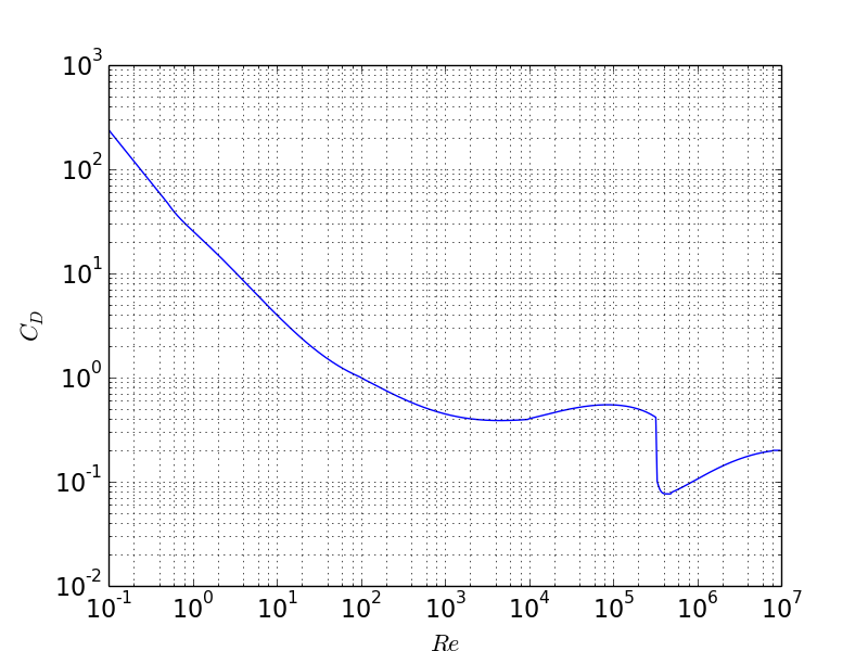
Figure 1 illustrates \( C_D \) as a function of \( Re \). The values in the plot are not as accurate as the number of digits in the program might indicate. For example is the location and the size of the "valley" in the diagram strongly dependent of the degree of turbulence in the free stream and the roughness of the sphere. As the drag coefficient \( C_D \) is a function of the Reynolds number, it is also a function of the solution \( v \) (i.e. the velocity) of the ODE in Equation (13). We will use the function \( C_D(Re) \) as an example of how functions may be implemented in Python.