Differences

We will study some simple methods to solve initial value problems. Later we shall see that these methods also may be used to solve boundary value problems for ODEs.

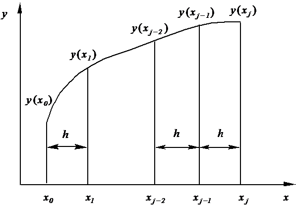
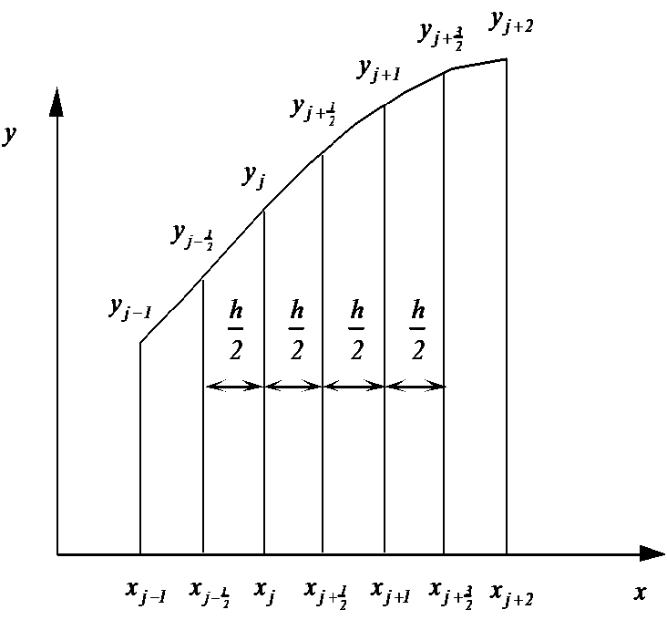
$$ \begin{equation*} x_j=x_0+jh \end{equation*} $$ where $ h=\Delta x $ is assumed constant unless otherwise stated.

Figure 2: Illustration of how to obtain difference equations.

Forward differences: $$ \begin{equation*} \Delta y_j=y_{j+1}-y_j \end{equation*} $$

Backward differences: $$ \begin{equation} \tag{15} \nabla y_j=y_j-y_{j-1} \end{equation} $$

Central differences: $$ \begin{equation*} \delta y_{j+\frac{1}{2}}=y_{j+1}-y_j \end{equation*} $$

The linear difference operators $ \Delta $, $ \nabla $ and $ \delta $ are useful when we are deriving more complicated expressions. An example of usage is as follows, $$ \begin{equation*} \delta ^2y_j=\delta (\delta y_j)=\delta (y_{1+\frac{1}{2}}-y_{1-\frac{1}{2}}) =y_{j+1}-y_j-(y_j-y_{j-1})=y_{j+1}-2y_j+y_{j-1} \end{equation*} $$

We will mainly write out the formulas entirely instead of using operators.

We shall find difference formulas and need again Taylor's theorem: $$ \begin{align} \tag{16} y(x)=&y(x_0)+y'(x_0)\cdot (x-x_0)+\frac{1}{2}y''(x_0)\cdot (x-x_0)^2 + \\ &\dots + \frac{1}{n!}y^{(n)}(x_0)\cdot (x-x_0)^n +R_n \nonumber \end{align} $$

The remainder $ R_n $ is given by $$ \begin{align} R_n&=\frac{1}{(n+1)!}y^{(n+1)}(\xi)\cdot (x-x_0)^{n+1}\\ &\text{where } \xi \in (x_0,x) \nonumber \end{align} $$

By use of (16) we get $$ \begin{align} \tag{17} y(x_{j+1}) \equiv &y(x_j+h)=y(x_j)+hy'(x_j) +\frac{h^2}{2}y''(x_j)+\\ &\dots+\frac{h^ny^{(n)}(x_j)}{n!}+R_n \nonumber \end{align} $$ where the remainder $ R_n=O(h^{n+1}),\ h\to 0 $.

From (17) we also get $$ \begin{equation} \tag{18} y(x_{j-1}) \equiv y(x_j-h)=y(x_j)-hy'(x_j)+\frac{h^2}{2}y''(x_j)+\dots+\frac{h^k(-1)^ky^{(k)}(x_j)}{k!}+\dots \end{equation} $$

We will here and subsequently assume that $ h $ is positive.

We solve (17) with respect to $ y' $: $$ \begin{equation} \tag{19} y'(x_j)=\frac{y(x_{j+1})-y(x_j)}{h}+O(h) \end{equation} $$

We solve (18) with respect to $ y' $: $$ \begin{equation} \tag{20} y'(x_j)=\frac{y(x_{j})-y(x_{j-1})}{h}+O(h) \end{equation} $$

By addition of (18) and (17) we get $$ \begin{equation} \tag{21} y''(x_j)=\frac{y(x_{j+1})-2y(x_{j})+y(x_{j-1})}{h^2}+O(h^2) \end{equation} $$

By subtraction of (18) from (17) we get $$ \begin{equation} \tag{22} y'(x_j)=\frac{y(x_{j+1})-y(x_{j-1})}{2h}+O(h^2) \end{equation} $$

Notation: We let $ y(x_j) $ always denote the function $ y(x) $ with $ x=x_j $. We use $ y_j $ both for the numerical and analytical value. Which is which will be implied.

Equations (19), (20), (21) and (22) then gives the following difference expressions: $$ \begin{align} \tag{23} &y'_j=\frac{y_{j+1}-y_j}{h}\ ;\ \text{truncation error}\ O(h)\\ \tag{24} &y'_j=\frac{y_{j}-y_{j-1}}{h}\ ;\ \text{truncation error}\ O(h)\\ \tag{25} &y''_j=\frac{y_{j+1}-2y_j+y_{j-1}}{h^2}\ ;\ \text{truncation error}\ O(h^2)\\ \tag{26} &y'_j=\frac{y_{j+1}-y_{j-1}}{2h}\ ;\ \text{truncation error}\ O(h^2) \end{align} $$

(23) is a forward difference, (24) is a backward difference while (25) and (26) are central differences.

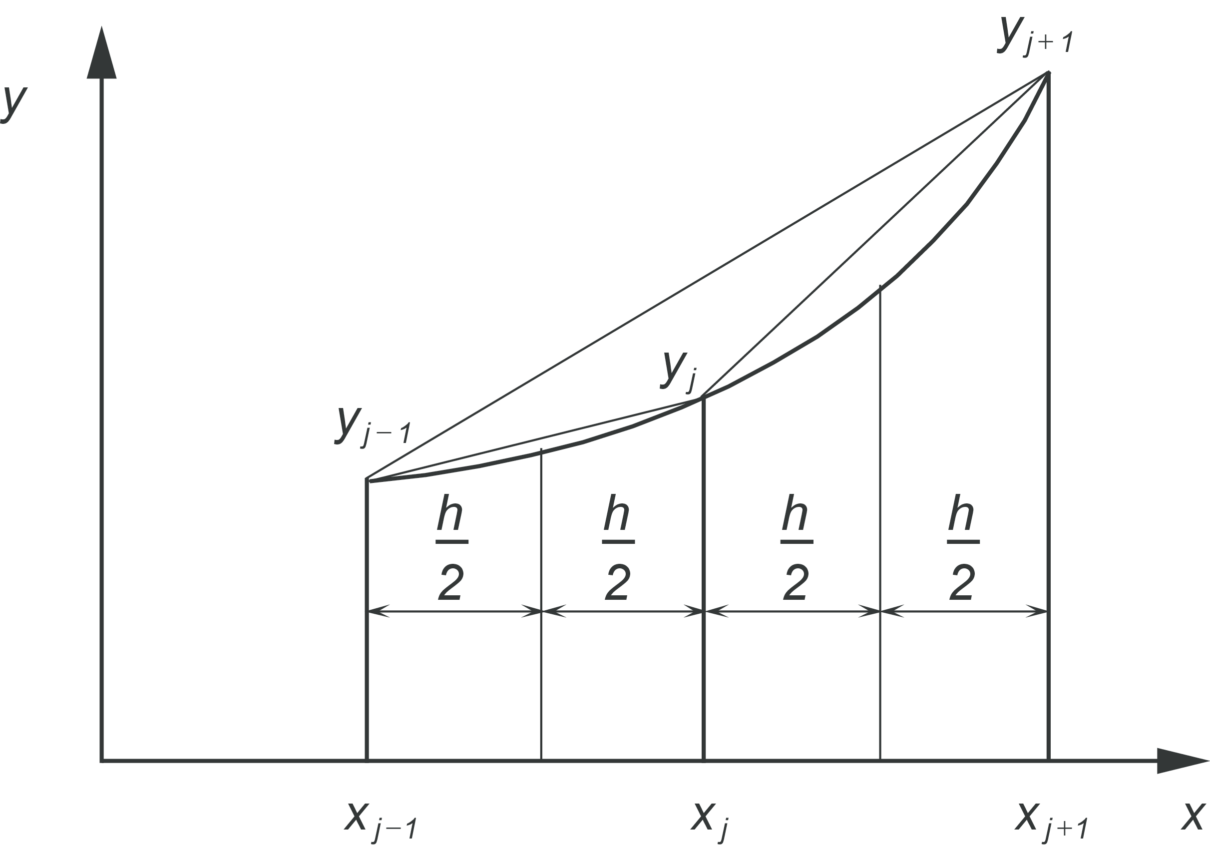
The expressions in (23), (24), (25) and (26) are easily established from the figure.

(23) follows directly.

(25): $$ \begin{equation*} y''_j(x_j)=\left(\frac{y_{j+1}-y_j}{h}-\frac{y_{j}-y_{j-1}}{h}\right)\cdot \frac{1}{h} = \frac{y_{j+1}-2y_j+y_{j-1}}{h^2} \end{equation*} $$

(26): $$ \begin{equation*} y'_j=\left(\frac{y_{j+1}-y_j}{h}-\frac{y_{j}+y_{j-1}}{h}\right)\cdot \frac{1}{2}=\frac{y_{j+1}-y_{j-1}}{2h} \end{equation*} $$

To find the truncation error we must use the Taylor series expansion.

The derivation above may be done more systematically. We set $$ \begin{equation} \tag{27} y'(x_j)=a\cdot y(x_{j-1})+b\cdot y(x_j)+c\cdot y(x_{j+1})+O(h^m) \end{equation} $$ where we shall determine the constants $ a $, $ b $ and $ c $ together with the error term. For simplicity we use the notation $ y_j\equiv y(x_j),\ y'_j \equiv y'(x_j) $ and so on. From the Taylor series expansion in (17) and (18) we get $$ \begin{align*} &a\cdot y_{j-1}+b\cdot y_j +c\cdot y_{j+1} = \\ &a\cdot\left[y_j-hy'_j+\frac{h^2}{2}y''_j+\frac{h^3}{6}y'''_j(\xi)\right]+b\cdot y_j + \\ &c\cdot \left[y_j-hy'_j+\frac{h^2}{2}y''_j+\frac{h^3}{6}y'''_j(\xi)\right] \end{align*} $$ Collecting terms: $$ \begin{align*} a\cdot y_{j-1}+b\cdot y_j +c\cdot y_{j+1} = \\ (a+b+c)y_j+(c-a)hy'_j+ \\ (a+c)\frac{h^2}{2}y''_j+(c-a)\frac{h^3}{6}y'''(\xi) \end{align*} $$ We determine $ a $, $ b $ and $ c $ such that $ y'_j $ gets as high accuracy as possible: $$ \begin{align} a+b+c=0 \nonumber \\ (c-a)\cdot h=1 \tag{28}\\ \nonumber a+c=1 \end{align} $$ The solution to (28) is $$ \begin{equation*} a=-\frac{1}{2h},\ b=0 \text{ and } c=\frac{1}{2h} \end{equation*} $$ which when inserted in (27) gives $$ \begin{equation} \tag{29} y'_j=\frac{y_{j+1}-y_{j-1}}{2h}-\frac{h^2}{6}y'''(\xi) \end{equation} $$ Comparing (29) with (27) we see that the error term is $ O(h^m)=-\frac{h^2}{6}y'''(\xi) $, which means that $ m=2 $. As expected, (29) is identical to (22).

Let's use this method to find a forward difference expression for $ y'(x_j) $ with accuracy of $ O(h^2) $. Second order accuracy requires at least three unknown coefficients. Thus, $$ \begin{equation} \tag{30} y'(x_j)=a\cdot y_j + b\cdot y_{j+1} + c\cdot y_{j+2} + O(h^m) \end{equation} $$ The procedure goes as in the previous example as follows, $$ \begin{align*} a&\cdot y_{j}+b\cdot y_{j+1} +c\cdot y_{j+2} =\\ a&\cdot y_j+b\cdot\left[y_j+hy'_j+\frac{h^2}{2}y''_j+\frac{h^3}{6}y'''(\xi)\right]+\\ c&\cdot \left[y_j+2hy'_j+2h^2y''_j+\frac{8h^3}{6}y'''_j(\xi)\right]\\ =&(a+b+c)\cdot y_j+(b+2c)\cdot hy'_j \\ +& h^2\left(\frac{b}{2}+2c\right)\cdot y''_j+\frac{h^3}{6}(b+8c)\cdot y'''(\xi) \end{align*} $$ We determine $ a $, $ b $ and $ c $ such that $ y'_j $ becomes as accurate as possible. Then we get, $$ \begin{align} a+b+c=0 \nonumber\\ (b+2c)\cdot h=1 \tag{31}\\ \frac{b}{2}+2c=0\nonumber \end{align} $$ The solution of (31) is $$ \begin{equation*} a=-\frac{3}{2h},\ b=\frac{2}{h},\ c=-\frac{1}{2h}\ \end{equation*} $$ which inserted in (30) gives $$ \begin{equation} \tag{32} y'_j=\frac{-3y_j+4y_{j+1}-y_{j+2}}{2h}+\frac{h^2}{3}y'''(\xi) \end{equation} $$ The error term $ O(h^m)=\frac{h^2}{3}y'''(\xi) $ shows that $ m=2 $.

Here follows some difference formulas derived with the procedure above:

Forward differences: $$ \begin{align*} \dfrac{dy_i}{dx}&=\dfrac{y_{i}-y_{i-1}}{\Delta x}+\dfrac{1}{2}y''(\xi)\Delta x \\ \dfrac{dy_i}{dx}&=\dfrac{3y_i-4y_{i-1}+y_{i-2}}{2\Delta x}+\dfrac{1}{3}y'''(\xi)\cdot (\Delta x)^2 \\ \dfrac{dy_i}{dx}&=\dfrac{11y_i-18y_{i-1}+9y_{i-2}-y_{i-3}}{6\Delta x}+\dfrac{1}{4}y^{(4)}(\xi)\cdot (\Delta x)^3 \\ \dfrac{d^2y_i}{dx^2}&=\dfrac{y_i-2y_{i-1}+y_{i-2}}{(\Delta x)^2}+y'''(\xi)\cdot \Delta x \\ \dfrac{d^2y_i}{dx^2}&=\dfrac{2y_i-5y_{i-1}+4y_{i-2}-y_{i-3}}{(\Delta x)^2}+\dfrac{11}{12}y^{(4)}(\xi)\cdot (\Delta x)^2 \end{align*} $$

Backward differences: $$ \begin{align*} \dfrac{dy_i}{dx}&=\dfrac{y_{i}-y_{i-1}}{\Delta x}+\dfrac{1}{2}y''(\xi)\Delta x \\ \dfrac{dy_i}{dx}&=\dfrac{3y_i-4y_{i-1}+y_{i-2}}{2\Delta x}+\dfrac{1}{3}y'''(\xi)\cdot (\Delta x)^2 \\ \dfrac{dy_i}{dx}&=\dfrac{11y_i-18y_{i-1}+9y_{i-2}-y_{i-3}}{6\Delta x}+\dfrac{1}{4}y^{(4)}(\xi)\cdot (\Delta x)^3 \\ \dfrac{d^2y_i}{dx^2}&=\dfrac{y_i-2y_{i-1}+y_{i-2}}{(\Delta x)^2}+y'''(\xi)\cdot \Delta x \\ \dfrac{d^2y_i}{dx^2}&=\dfrac{2y_i-5y_{i-1}+4y_{i-2}-y_{i-3}}{(\Delta x)^2}+\dfrac{11}{12}y^{(4)}(\xi)\cdot (\Delta x)^2 \end{align*} $$

Central differences: $$ \begin{align*} \dfrac{dy_i}{dx}&=\dfrac{y_{i+1}-y_{i-1}}{2\Delta x}-\dfrac{1}{6}y'''(\xi)(\Delta x)^2 \\ \dfrac{dy_i}{dx}&=\dfrac{-y_{i+2}+8y_{i+1}-8y_{i-1}+y_{i-2}}{12\Delta x}+\dfrac{1}{30}y^{(5)}(\xi)\cdot (\Delta x)^4 \\ \dfrac{d^2y_i}{dx^2}&=\dfrac{y_{i+1}-2y_{i}+y_{i-1}}{(\Delta x)^2}-\dfrac{1}{12}y^{(4)}(\xi)\cdot (\Delta x)^2 \\ \dfrac{d^2y_i}{dx^2}&=\dfrac{-y_{i+2}+16y_{i+1}-30y_{i}+16y_{i-1}-y_{i-2}}{12(\Delta x)^2}+\dfrac{1}{90}y^{(6)}(\xi)\cdot (\Delta x)^4 \\ \dfrac{d^3y_i}{dx^3}&=\dfrac{y_{i+2}-2y_{i+1}+2y_{i-1}-y_{i-2}}{2(\Delta x)^3}+\dfrac{1}{4}y^{(5)}(\xi)\cdot (\Delta x)^2 \end{align*} $$