Visual exploration
This section explains how to load the data from the computation, stored
as a pickled list in the file bumpy.res, into various arrays, and how
to visualize these arrays. We want to produce the following plots:
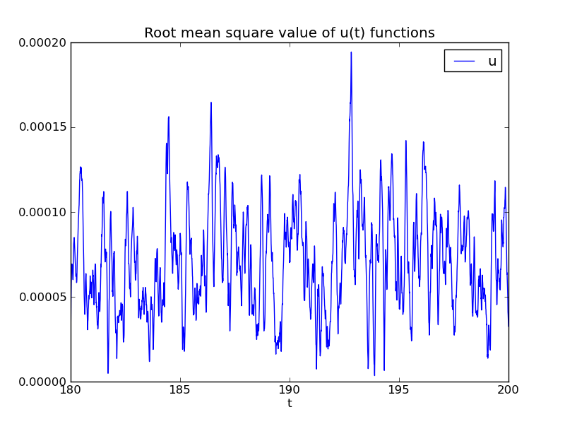
- the root mean square value of \( u(t) \), to see the typical amplitudes
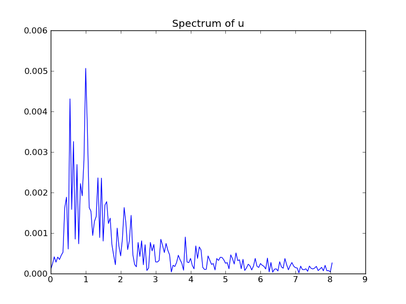
- the spectrum of \( u(t) \), for \( t>t_s \) (using FFT) to see which frequencies that dominate in the signal
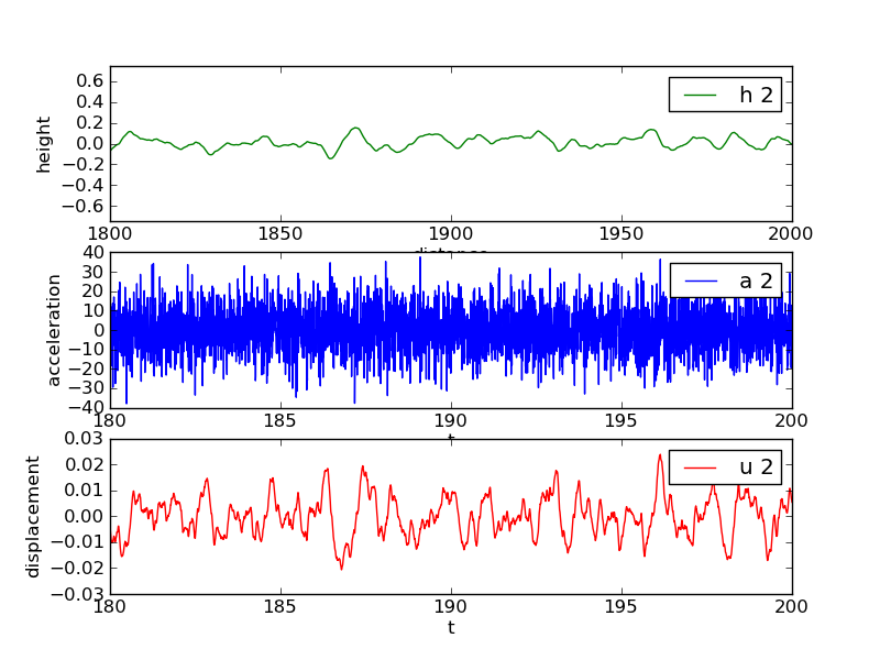
- for each road shape, a plot of \( h(x) \), \( a(t) \), and \( u(t) \), for \( t\geq t_s \)
pylab module for curve plotting since it provides
a syntax very close to that of MATLAB, which is well known by many readers.
from matplotlib.pylab import *
This import also perform as from numpy import * such that we have access
to all the array functionality too.
Loading the computational data from file back to a list data is done
by
import cPickle
outfile = open('bumpy.res', 'r')
data = cPickle.load(outfile)
outfile.close()

x, t = data[0:2]
u_rms = data[-1]
The remaining data, data[2:-1], contains all the 3-lists [h, a, u]
from the computations in the function forced_vibrations.
Since now we concentrate on the part \( t\geq t_s \) of the data, we can grab the corresponding parts of the arrays in the following way, using boolean arrays as indices:
indices = t >= t_s   # True/False boolean array
t = t[indices]       # fetch the part of t for which t > t_s
x = x[indices]       # fetch the part of x for which t > t_s
Indexing by a boolean array extracts all the elements corresponding to
the True elements in the index array.
Plotting the root mean square value array u_rms for t >= t_s is now done by
figure()
u_rms = u_rms[indices]
plot(t, u_rms)
legend(['u'])
xlabel('t')
title('Root mean square value of u(t) functions')
Figure 3 shows the result.
The spectrum of a \( u(t) \) function (represented through the arrays u
and t) can be computed by the Python function
def frequency_analysis(u, t):
    A = fft(u)
    A = 2*A
    dt = t[1] - t[0]
    N = t.size
    freq = arange(N/2, dtype=float)/N/dt
    A = abs(A[0:freq.size])/N
    # Remove small high frequency part
    tol = 0.05*A.max()
    for i in xrange(len(A)-1, 0, -1):
        if A[i] > tol:
            break
    return freq[:i+1], A[:i+1]
Note here that we truncate that last part of the spectrum where the amplitudes are small (this usually gives a plot that is easier to inspect).
In the present case, we utilize the frequency_analysis through
figure()
u = data[3][2][indices]  # 2nd realization of u
f, A = frequency_analysis(u, t)
plot(f, A)
title('Spectrum of u')
Note the list look-up data[3][2][indices]: the element with index
3 contains the 2nd 3-list [h, a, u], and the element with index 2
in this 3-list is the u array, in which we seek the part where
\( t\geq t_s \), here corresponding to the True indices in the boolean
array indices.
Figure 4 shows the amplitudes and that the dominating frequency is 1 Hz.
Finally, we can run through all the 3-lists [h, a, u] and plot
these arrays:
case_counter = 0
for h, a, u in data[2:-1]:
    h = h[indices]
    a = a[indices]
    u = u[indices]

    figure()
    subplot(3, 1, 1)
    plot(x, h, 'g-')
    legend(['h %d' % case_counter])
    hmax = (abs(h.max()) + abs(h.min()))/2
    axis([x[0], x[-1], -hmax*5, hmax*5])
    xlabel('distance'); ylabel('height')

    subplot(3, 1, 2)
    plot(t, a)
    legend(['a %d' % case_counter])
    xlabel('t'); ylabel('acceleration')

    subplot(3, 1, 3)
    plot(t, u, 'r-')
    legend(['u %d' % case_counter])
    xlabel('t'); ylabel('displacement')
    savefig('tmp%d.png' % case_counter)
    case_counter += 1
Figure 5: First realization of a bumpy road, with corresponding acceleration of the wheel and resulting vibrations.
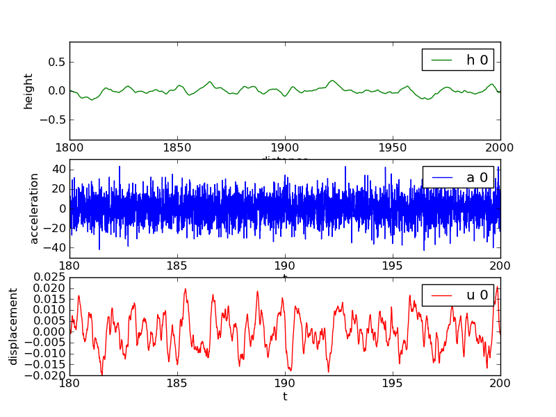
Figure 6: Second realization of a bumpy road, with corresponding acceleration of the wheel and resulting vibrations.
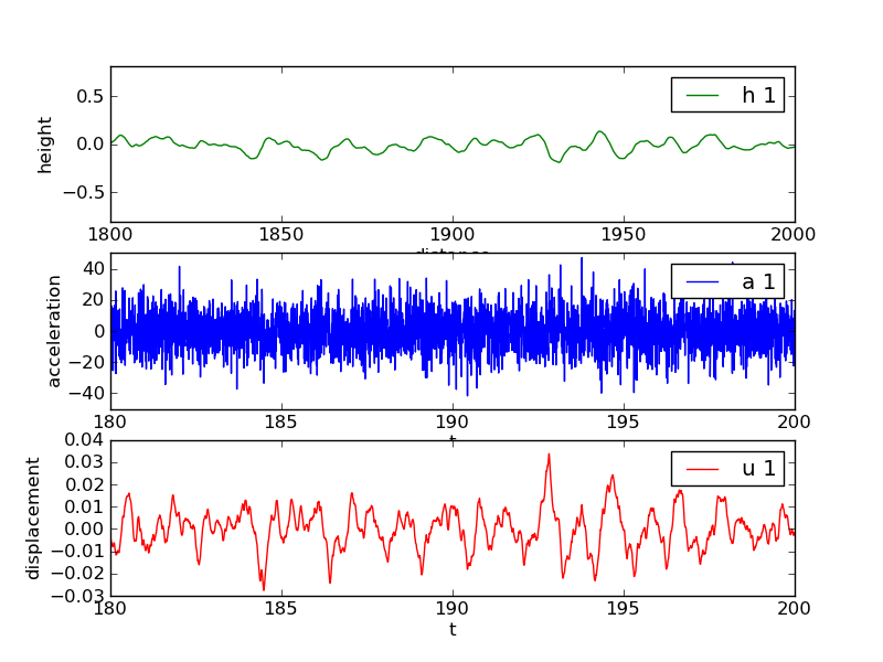
Figure 7: Third realization of a bumpy road, with corresponding acceleration of the wheel and resulting vibrations.
If all the plot commands above are placed in a file, as in
explore.py, a final show() call is needed to show the
plots on the screen. On the other hand, the commands are usually
more conveniently performed in an interactive Python shell, preferably
IPython.
Advanced topics
Symbolic computing via SymPy
Python has a package SymPy that offers symbolic computing. Here is a simple introductory example where we differentiate a quadratic polynomial, integrate it again, and find the roots:
>>> import sympy as sp
>>> x, a = sp.symbols('x a')        # Define mathematical symbols
>>> Q = a*x**2 - 1                  # Quadratic function
>>> dQdx = sp.diff(Q, x)            # Differentiate wrt x
>>> dQdx
2*a*x
>>> Q2 = sp.integrate(dQdx, x)      # Integrate (no constant)
>>> Q2
a*x**2
>>> Q2 = sp.integrate(Q, (x, 0, a)) # Definite integral
>>> Q2
a**4/3 - a
>>> roots = sp.solve(Q, x)          # Solve Q = 0 wrt x
>>> roots
[-sqrt(1/a), sqrt(1/a)]
One can easily convert a SymPy expression like Q into
a Python function Q(x, a) to be used for further numerical
computing:
>>> Q = sp.lambdify([x, a], Q)      # Turn Q into Py func.
>>> Q(x=2, a=3)                     # 3*2**2 - 1 = 11
11
Sympy can do a lot of other things. Here is an example on computing the Taylor series of \( e^{-x}\sin(rx) \), where \( r \) is the smallest root of \( Q=ax^2-1=0 \) as computed above:
>>> f = sp.exp(-a*x)*sp.sin(roots[0]*x)
>>> f.series(x, 0, 4)
-x*sqrt(1/a) + x**3*(-a**2*sqrt(1/a)/2 + (1/a)**(3/2)/6) +
a*x**2*sqrt(1/a) + O(x**4)
Testing
Software testing in Python is best done with a unit test framework
such as nose or pytest. These frameworks can automatically
run all functions starting with test_ recursively in files in a
directory tree. Each test_* function is called a test function
and must take no arguments and apply assert to a boolean expression
that is True if the test passes and False if it fails.
Example on a test function
def halve(x):
    """Return half of x."""
    return x/2.0

def test_halve():
    x = 4
    expected = 2
    computed = halve(x)
    # Compare real numbers using tolerance
    tol = 1E-14
    diff = abs(computed - expected)
    assert diff < tol
Test function for the numerical solver
A frequently used technique to test differential equation solvers is to just specify a solution and fit a source term in the differential equation such that the specified solution solves the equation. The initial conditions must be set according to the specified solution. This technique is known as the method of manufactured solutions.
Here we shall specify a solution that is quadratic or linear
in \( t \) because
such lower-order polynomials will often be an exact solution of both
the differential equation and the finite difference equations.
This means that the polynomial should be reproduced to machine
precision by our solver function.
We can use SymPy to find an appropriate \( F(t) \) term in the differential equation such that a specified solution \( u(t)=I + Vt + qt^2 \) fits the equation and initial conditions. With quadratic damping, only a linear \( u \) will solve the discrete equation so in this case we choose \( u=I+Vt \).
We embed the SymPy calculations and the numerical calcuations in a test function:
def lhs_eq(t, m, b, s, u, damping='linear'):
    """Return lhs of differential equation as sympy expression."""
    v = sm.diff(u, t)
    d = b*v if damping == 'linear' else b*v*sm.Abs(v)
    return m*sm.diff(u, t, t) + d + s(u)

def test_solver():
    """Verify linear/quadratic solution."""
    # Set input data for the test
    I = 1.2; V = 3; m = 2; b = 0.9; k = 4
    s = lambda u: k*u
    T = 2
    dt = 0.2
    N = int(round(T/dt))
    time_points = np.linspace(0, T, N+1)

    # Test linear damping
    t = sm.Symbol('t')
    q = 2  # arbitrary constant
    u_exact = I + V*t + q*t**2   # sympy expression
    F_term = lhs_eq(t, m, b, s, u_exact, 'linear')
    print 'Fitted source term, linear case:', F_term
    F = sm.lambdify([t], F_term)
    u, t_ = solver(I, V, m, b, s, F, time_points, 'linear')
    u_e = sm.lambdify([t], u_exact, modules='numpy')
    error = abs(u_e(t_) - u).max()
    tol = 1E-13
    assert error < tol

    # Test quadratic damping: u_exact must be linear
    u_exact = I + V*t
    F_term = lhs_eq(t, m, b, s, u_exact, 'quadratic')
    print 'Fitted source term, quadratic case:', F_term
    F = sm.lambdify([t], F_term)
    u, t_ = solver(I, V, m, b, s, F, time_points, 'quadratic')
    u_e = sm.lambdify([t], u_exact, modules='numpy')
    error = abs(u_e(t_) - u).max()
    assert error < tol
Appendix: Quick motivation for programming with Python
Appendix: Scientific Python resources
Full tutorials on scientific programming with Python
- Python Scientific Lecture Notes (from EuroSciPy tutorials, based on Python Scientific)
- Scientific Python Lectures as IPython notebooks
- Stefan van der Walt's lectures
NumPy resources
- NumPy Tutorial
- NumPy User Guide
- Advanced NumPy Tutorial
- Advanced NumPy Course
- NumPy Example List
- NumPy Medkit
- NumPy and SciPy Cookbook
- NumPy for Matlab Users
- NumPy for Matlab/R/IDL Users
Useful resources
- AstroPython
- Talk on IPython by Fernando Perez
- Useful software in the Scientific Python Ecosystem
- IPython
- Python(x,y)
- Basic Motion Graphics with Python
Some relevant Python books
- Think Python
- Learn Python The Hard Way
- Dive Into Python
- Think Like a Computer Scientist
- Introduction to Python Programming (for scientists)
- A Primer on Scientific Programming with Python
- Gerard Gorman has made associated IPython notebooks for teaching
- Traditional beamer slides are also available
- Python Scripting for Computational Science
Course material on Python programming in general
- The Official Python Tutorial
- Python Tutorial on tutorialspoint.com
- Interactive Python tutorial site
- A Beginner's Python Tutorial on wikibooks.org
- Python Programming on wikibooks.org
- Non-Programmer's Tutorial for Python on wikibooks.org
- Python For Beginners
- Gentle Python introduction for high school (with associated IPython notebooks)
- A Gentle Introduction to Programming Using Python (MIT OpenCourseWare)
- Introduction to Computer Science and Programming (MIT OpenCourseWare with videos)
- Learning Python Programming Language Through Video Lectures
- Python Programming Tutorials Video Lecture Course (Learners TV)
- Python Videos, Tutorials and Screencasts